6  Structure of Empirical Networks

Introduction

So far, we’ve introduced several ways to quantify and visualize the properties of networks. Many of our examples have been small, and we’ve used the same network several times to illustrate important points. In this chapter, we’ll address an important empirical question:

What are some of the properties of real networks more broadly?

Of course, there’s no simple answer to this question: we observe network data sets across a wide variety of domains, and many of them have different properties. For our purposes today, we’ll look at a sample of four networks, including two familiar ones provided with NetworkX and two new ones:

• twitch: A network of mutual friends on the Twitch streaming platform. The data set was collected by Rozemberczki, Allen, and Sarkar (2021).
• chameleon: A network of Wikipedia pages on topics related to chameleons (yes, the animal). An edge exists between two nodes if the corresponding Wikipedia pages link to each other. The data set was collected by Rozemberczki, Allen, and Sarkar (2021).
• karate: The Zachary Karate Club social network (Zachary 1977), which is packaged with NetworkX.
• les_mis: A network of character interactions in the novel Les Miserables by Victor Hugo, also packaged with NetworkX.
• org_1 and org_2: Two anonymized Facebook social networks of employees in two different mediums-sized organizations. This data was collected and published by Fire and Puzis (2012). Nodes are employees and edges are friendships. This data set was accessed from the website of Michael Fire and discovered via the Colorado Index of Complex Networks (ICON).

Our first task is to download these data sets and read them in as NetworkX graph objects, which we do in the hidden cell below.

from matplotlib import pyplot as plt
import networkx as nx
plt.style.use('seaborn-v0_8-whitegrid')
import numpy as np
from scipy.special import factorial
import pandas as pd
import random

# acquire twitch data
url = "https://raw.githubusercontent.com/benedekrozemberczki/MUSAE/master/input/edges/ENGB_edges.csv"
edges = pd.read_csv(url)
G_twitch = nx.from_pandas_edgelist(edges, "from", "to", create_using=nx.Graph)

# acquire chameleon data
url = "https://raw.githubusercontent.com/benedekrozemberczki/MUSAE/master/input/edges/chameleon_edges.csv"
edges = pd.read_csv(url)
G_chameleon = nx.from_pandas_edgelist(edges, "id1", "id2", create_using=nx.Graph)

# acquire organizations data

url = "https://raw.githubusercontent.com/network-science-notes/network-science-notes.github.io/refs/heads/main/data/organization-social-networks/M1Anonymized.csv"
edges = pd.read_csv(url, header=None)
G_org_1 = nx.from_pandas_edgelist(edges, 0, 1, create_using=nx.Graph)

url = "https://raw.githubusercontent.com/network-science-notes/network-science-notes.github.io/refs/heads/main/data/organization-social-networks/M2Anonymized.csv"
edges = pd.read_csv(url, header=None)
G_org_2 = nx.from_pandas_edgelist(edges, 0, 1, create_using=nx.Graph)

# two built-in networkx data sets. 
G_karate = nx.karate_club_graph()
G_les_mis = nx.les_miserables_graph()

Now that we have our data sets, we could in principle go ahead and compute various measurements and properties. However, a fundamental principle in measuring networks is to compare. If we say that a network has a high value of some measurement \(X\), then the correct reply is:

High compared to what?

The following code constructs a random synthetic counterpart graph for each of our empirical graphs. It then adds all of these to a dictionary so that we can easily access both the real and synthetic graphs later.

def unweight(G):
    for source, target in G.edges():
        G[source][target]['weight'] = 1

def random_counterpart(G):
    degrees = [deg for (node, deg) in G.degree()]
    G_random = nx.expected_degree_graph(degrees, selfloops=False)
    G_random.remove_edges_from(nx.selfloop_edges(G_random))
    return G_random

def add_to_dataset_dict(dataset_dict, G, name):
    unweight(G)
    dataset_dict[name] = {
        "graph" : G,
        "random" : random_counterpart(G)
    }

Now we’ll prepare our dictionary of data sets.

dataset_dict = {}

for graph, name in {G_twitch: "twitch", 
                    G_chameleon: "chameleon", 
                    G_karate: "karate", 
                    G_les_mis: "les_mis", 
                    G_org_1: "org_1", 
                    G_org_2: "org_2"}.items():

    add_to_dataset_dict(dataset_dict, graph, name)

To help us compute and compare measurements on these graphs, we’ll define the following function which will manage these computations and organize the result as a table. This function takes as an argument a function fun which accepts a graph as an input and returns a scalar value.

def compute_metric(fun = lambda x: 0, compare = True):
    print("Data Set" + " " * 10 + "Real", end = "")
    if compare: 
            print(" " * 10 + "Random")
    else: 
        print()
    print("-" * 22, end = "")
    if compare: 
        print("-"*18)
    else: 
        print()
    for data_set in dataset_dict:
        print(data_set + " " * (14 - len(data_set)) + f"{fun(dataset_dict[data_set]['graph']):>8.2f}", end = "")
        if compare:
            print(" " * (8) + f"{fun(dataset_dict[data_set]['random']):>8.2f}")
        else: 
            print()

Clustering Coefficient

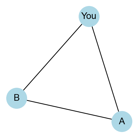
Now that we have our experimental setup in place, let’s move on to something more complex. Take a moment and think of two of your friends, whom we’ll call \(A\) and \(B\). Are \(A\) and \(B\) themselves friends with each other? If they are, then we say that you, \(A\), and \(B\) together form a triangle or triad in the social network.

A stylized fact about many networks—especially social networks—is that triangles like these are common. In order to validate this stylized fact, we need to (a) determine how to measure the prevalence of triangles and (b) compare the value of this measure on our real networks to that of their random counterparts.

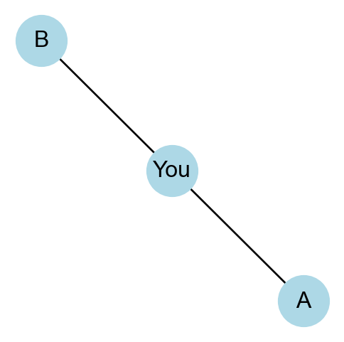
There are many possible measures of the prevalence of triangles, but here we will use the transitivity: the fraction of all possible triangles that are present in the network. We define a possible triangle as a path of length 3 like that shown in Figure 6.1; the addition of just a single edge would turn this path into a triangle.

It is possible to show that the number of possible triangles with node \(i\) in the middle is \(k_i(k_i - 1)/2\), where \(k_i\) is the degree of node \(i\). The transitivity is then the ratio of the number of triangles to the number of possible triangles.

\[ \begin{aligned} T(G) = \frac{\mathrm{trace}(\mathbf{A}^3)}{\sum_{i} k_i(k_i - 1)} \end{aligned} \]

Here, \(\mathbf{A}\) is the adjacency matrix of \(G\) and \(k_i\) is the degree of node \(i\).

Let’s write a function to compute the transitivity of a graph.

def my_transitivity(G):
    A = nx.adjacency_matrix(G).toarray()

    # numerator
    num_triangles = np.trace(A @ A @ A)

    # denominator
    degrees = A.sum(axis = 0)
    num_triplets = np.sum(degrees * (degrees - 1))

    return num_triangles / num_triplets

Let’s compare our function to the built-in function supplied by NetworkX.

print(my_transitivity(G_karate))
print(nx.transitivity(G_karate))

0.2556818181818182
0.2556818181818182

Looks good! We’ll move forward with the NetworkX version, as it is substantially faster on larger graphs.

compute_metric(nx.transitivity)

Data Set          Real          Random
----------------------------------------
twitch            0.04            0.03
chameleon         0.31            0.12
karate            0.26            0.26
les_mis           0.50            0.26
org_1             0.26            0.09
org_2             0.23            0.02

We observe that the chameleon and les_mis graphs appear to have substantially greater transitivity than their random counterparts, while both karate and twitch have similar transitivity to their random counterparts. The two organizational social networks have much higher transitivity than their random counterparts as well. Under this comparison, some networks indeed display very high transitivity. Indeed, it’s thought that most social networks have high transitivity.

When interpreting these results, it’s helpful to explicitly describe what is captured by the random counterpart when stating our conclusions. Recall that we constructed the random counterpart graphs to approximately preserve the degree sequence of the original data graph, while being otherwise random. Our conclusion could therefore be that graphs like chameleon, les_mis, or the two organizational graphs have higher values of the transitivity than can be explained by their degree sequences alone.

Degree-Degree Correlations

We have constructed random counterpart networks that have similar degree sequences to the real networks we are studying. Networks, however, can have interesting degree structures beyond just the degree sequence. One such structure is the degree-assortativity. The degree assortativity measures the extent to which nodes of similar degree are connected to each other. There are several ways to measure degree assortativity, but the most common one (due to Newman (2018)) has formula

\[ \begin{aligned} C = \frac{\sum_{(u,v) \in G} k_u k_v - \frac{1}{m}\left(\sum_{(u,v) \in G} k_u\right)^2}{\sum_{(u,v) \in G} k_u^2 - \frac{1}{m}\left(\sum_{(u,v) \in G} k_u\right)^2}\;. \end{aligned} \]

An assortative network (with high assortativity) is one in which nodes of high degree tend to connect to each other frequently. A disassortative network (with negative assortativity) is one in which nodes of high degree tend to connect to nodes of low degree. Let’s take a look at the assortativity values in our networks:

compute_metric(nx.degree_assortativity_coefficient)

Data Set          Real          Random
----------------------------------------
twitch           -0.12           -0.04
chameleon        -0.20           -0.06
karate           -0.48           -0.20
les_mis          -0.17           -0.00
org_1             0.11           -0.01
org_2             0.09           -0.01

The two organizational social networks are slightly assortative: employees have a tendency to associate with those who are similarly connected to them. On the other hand, the remaining networks are disassortative, even in comparison to their random counterparts.

Disassortativity is a common feature of many networks, and it is often attributed to the presence of hubs in the network. Hubs are nodes with very high degree, and they tend to connect to many other nodes. Since there are only a few hubs, they are more likely to connect to nodes of low degree than to other hubs.

Shortest Path Lengths

In a famous study, Stanley Milgram (1967) ¹ asked participants to ensure that a letter reached a target person, whom they did not know, in a US city. However, the participants were only allowed to send the letter to someone they knew on a first-name basis. That person could then send the letter to another person they knew on a first-name basis, and so on, until the letter was delivered (or lost). Perhaps surprisingly, many participants were able to reach the target person in only a few steps, on average. This experiment is the origin of the famous phrase six degrees of separation: in many social networks, most individuals are separated by relatively few links, even when the network is very large.

To test this in our networks, we’ll compute the length of the shortest path between a pair of nodes, averaged across all possible pairs. This quantity isn’t defined for the random counterpart networks that have multiple disconnected components (why?), and so we’ll stick to calculating it on the real-world networks.

compute_metric(nx.average_shortest_path_length, compare = False)

Data Set          Real
----------------------
twitch            3.68
chameleon         3.56
karate            2.41
les_mis           2.64
org_1             3.04
org_2             2.76

Indeed, despite some of these networks having thousands of nodes and edges, the average shortest path length does not exceed 4 links. We’ll consider some theoretical models that aim to explain this phenomenon later in the course.

Degree Distributions

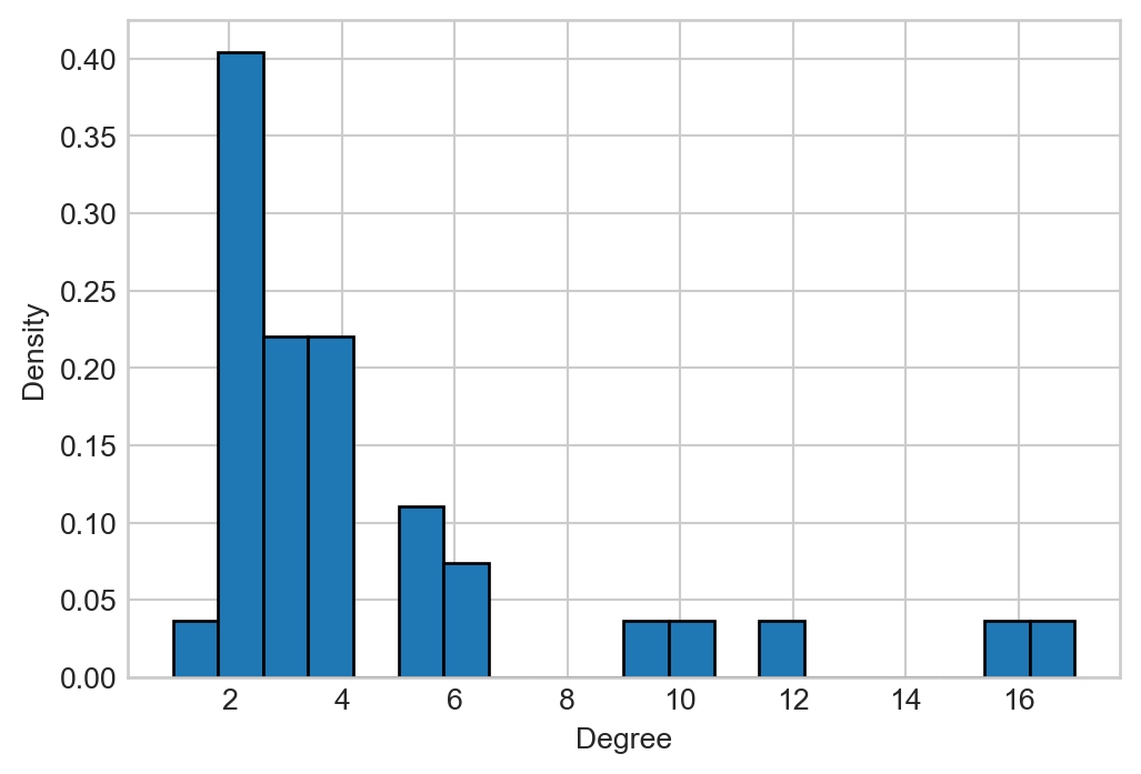
So far in our investigations, we’ve focused on comparing networks to randomized counterparts that have similar degrees. But what if we want to look at the degrees themselves? The way we most frequently do this is by analyzing the degree distribution, which we can think of as a histogram of the node degrees. Let’s look at the degree histogram for the karate club network:

Show code

fig, ax = plt.subplots(1, 1, figsize = (6, 4))
deg = np.array([deg for i, deg in nx.degree(G_karate)])
hist = ax.hist(deg, bins = 20, density = True,  edgecolor = "black")
ax.set(xlabel = "Degree", ylabel = "Density")

Heavy-tailed distributions are difficult to visualize on linear scales, so we often instead plot them on log-log scales. The helper functions in the hidden code cell below implement what is called “logarithmic binning” and plot the resulting log-binned histograms on logarithmic axes:

def log_binned_histogram(degree_sequence, interval = 5, num_bins = 20):
    hist, bins = np.histogram(degree_sequence, bins = min(int(len(degree_sequence)/interval), num_bins))
    bins = np.logspace(np.log10(bins[0]),np.log10(bins[-1]),len(bins))
    hist, bins = np.histogram(degree_sequence, bins = bins)
    binwidths = bins[1:] - bins[:-1]
    hist = hist / binwidths
    p = hist/hist.sum()
    return bins[:-1], p

def plot_degree_distribution(G, ax, **kwargs):

    deg_seq = np.array([deg for i, deg in nx.degree(G)])
    x, p = log_binned_histogram(deg_seq, **kwargs)
    ax.scatter(x, p,  facecolors='none', edgecolors =  'cornflowerblue', linewidth = 2, label = "Data")
    ax.loglog()

We can use these functions to plot the degree distribution of the networks we’ve previously studied:

Show code

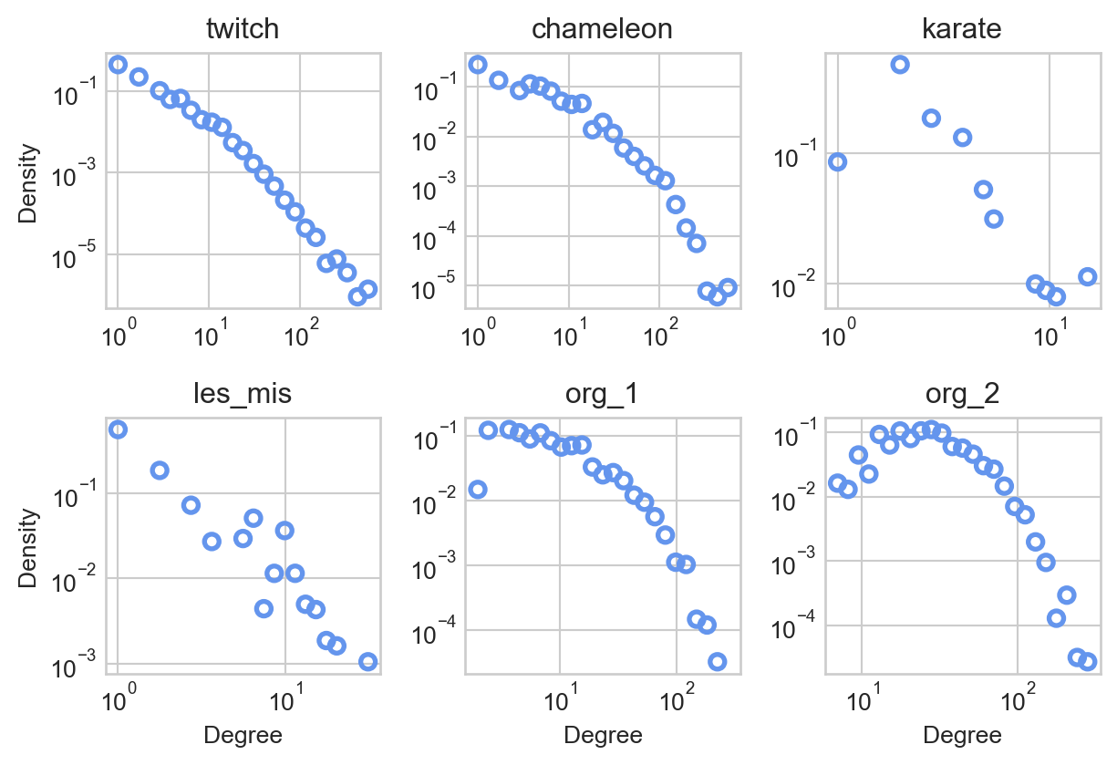
fig, ax = plt.subplots(2, 3, figsize = (6.5, 4.5))

for i, name in enumerate(dataset_dict): 
    
    plot_degree_distribution(dataset_dict[name]["graph"], ax.ravel()[i], interval = 1, num_bins = 25)
    ax.ravel()[i].set_title(name)

    if i % 3 == 0: 
        ax.ravel()[i].set(ylabel = "Density")
    if i >= 3:
        ax.ravel()[i].set(xlabel = "Degree")

plt.tight_layout()

Comparing our different data sets, we can observe a range of shapes in the degree distributions. One especially interesting feature of degree distributions that has received a LOT of attention in the networks literature (Holme (2019)) is the roughly linear behavior on log-log axes displayed, among our data sets, by the twitch graph. If we remember that both the horizontal and vertical axes are logarithmic, apparent linearity on these log-log axes corresponds to the equation

\[ \begin{aligned} \log p_k = \log C - \gamma \log k\;, \end{aligned} \]

where \(p_k\) is the proportion of nodes with degree \(k\) and \(C\) and \(\gamma\) are constants. Exponentiating both sides gives

\[ \begin{aligned} p_k = C k^{-\gamma}\;, \end{aligned} \tag{6.1}\]

which is called a power law for degree distribution. We say that the degree distribution of the twitch network appears to obey a power law in the tail of the distribution, since the linear behavior is only visible for larger values of \(k\).