In the last lecture, we discovered that the notion of connectivity could tell us something important about graph structure.
Components
Many networks have parts that are disconnected from each other. These parts are called components. As we saw in an example from the previous lecture, there is no path between any pair of nodes in different components of a network. In undirected graphs, the definition of connected components is relatively simple.
Definition 3.1 (Connected Components in an Undirected Graph) Two nodes \(i\) and \(j\) are path-connected if there exists a path between \(i\) and \(j\). The set \(\{j \in V : i \text{ is path-connected to } j\}\) is called the connected component of \(i\). A graph is connected if it has only one connected component. Otherwise, we say the network is disconnected.
For the purposes of this definition, we say that every node \(i\) has a zero-length path to itself. It follows that a singleton (a node with no edges attached) is its own connected component.
Exercise
Prove that the relation \(~\) defined as \(i ~ j\) iff there exists a path between \(i\) and \(j\) is an equivalence relation. Prove also that the equivalence classes of this relation are exactly the connected components of \(G\).
As we saw with degree, the definition of connected components requires a bit more subtlety when we consider directed networks.
Definition 3.2 (Strongly and Weakly Connected Components) In a directed network, two nodes \(i\) and \(j\) are strongly connected if there exists a path from \(i\) to \(j\) and a path from \(j\) to \(i\). Nodes \(i\) and \(j\) are weakly connected if there exists either a path from \(i\) to \(j\) or from \(j\) to \(i\).
The set \(\{j \in V : i \text{ is strongly connected to } j\}\) is called the strongly connected component of \(i\), and the set \(\{j \in V : i \text{ is weakly connected to } j\}\) is called the weakly connected component of \(i\).
A directed graph is strongly connected if it has only one strongly connected component. A directed graph is weakly connected if it is not strongly connected and has only one weakly connected component.
Two strongly connected nodes are also weakly connected.Intuitively, a weakly connected component is a connected component in the undirected version of the directed graph in which we “forget” the directionality of the edges.
Exercise
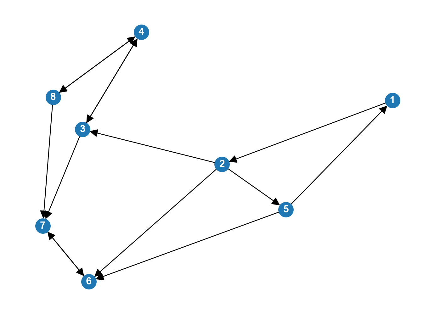
Identify the strongly connected components and the weakly connected components in the network below.
In directed networks, we can also define individual node properties that describe all nodes that could reach or be reached by our node of interest.
Definition 3.3 The in-component of node \(i\) is the set of nodes \(\{j \in V : \text{ there is a directed path from } i \text{ to } j\}\).
The out-component of node \(i\) is the set of nodes \(\{j \in V : \text{ there is a directed path from } j \text{ to } i\}\)
As with connected components, we include the node \(i\) itself as a member of its own in- and out-components.
Exercise
Let \(C^{\mathrm{in}}(i)\) and \(C^{\mathrm{out}}(i)\) be the in-component and out-component of node \(i\) in a directed network. Describe the sets \(C^{\mathrm{in}}(i) \cap C^{\mathrm{out}}(i)\) and \(C^{\mathrm{in}}(i) \cup C^{\mathrm{out}}(i)\) in vocabulary we have previously introduced.
The Graph Laplacian
We now introduce the graph Laplacian. The Laplacian is a matrix representation of a network that is surprisingly useful in a wide variety of applications. With our focus on components today, we’ll find an especially striking property of the Laplacian: the eigenvalues of the Laplacian give us a guide to the connected component structure of a graph.
There are multiple matrices that use this name; the one we introduce here is sometimes called the combinatorial graph Laplacian.The Laplacian is also useful in studying random walks and dynamics, for clustering and data analysis, for graph visualization, partitioning, and more!
Definition 3.4 (Laplacian of an Undirected Graph) The (combinatorial) graph Laplacian \(L\) of an undirected graph with adjacency matrix \(A\) is
\[
{\bf L} = {\bf D} - {\bf A} \,
\]
where \({\bf D}\) is the diagonal matrix whose diagonal entries \(D_{ii} = k_i\) contain the degree of node \(i\). An individual entry of the Laplacian can be written
We observe that the diagonal of the Laplacian gives the degrees of each node (from the matrix \(\mathbf{D}\)), while the off diagonal entries give the negatives of the entries of the adjacency matrix.
Definition 3.4 generalizes in a straightforward way for weighted networks with positive weights. There are also variants for directed graphs (including using in-degree or out-degree matrices to build an in-degree Laplacian or an out-degree Laplacian); not all of the properties we describe below hold for these variants.
Properties of the Graph Laplacian
We now investigate the mathematical properties of the graph Laplacian. We’ll leave proofs of many of these properties as exercises. Throughout, this section, let \(\mathbf{L} \in \mathbb{R}^{n\times n}\) be the combinatorial Laplacian matrix of a graph \(G\) on \(n\) nodes, and let \(\mathbf{1} \in \mathbb{R}^n\) be the vector of ones.
Theorem 3.1 (Elementary Properties of the Graph Laplacian)
\({\bf L}\) is real and symmetric.
The eigenvalues of \(\mathbf{L}\) are all real.
\({\bf L}{\bf 1} = {\bf 0}.\) That is, every row sums to 0.
Another important property of the Laplacian is that it is positive semi-definite.
Theorem 3.2 (Positive-semidefiniteness of the Laplacian) For any \(\mathbf{x} \in \mathbb{R}^n\), it holds that \(\mathbf{x}^T\mathbf{Lx} \geq 0\).
Because the Laplacian is symmetric, this is equivalent to:
Theorem 3.3 (The Laplacian has nonnegative eigenvalues) If \(\lambda\) is an eigenvalue of the Laplacian \(\mathbf{L}\), then \(\lambda \geq 0\).
Can we get more specific about the spectral structure of the eigenvalues? In fact, we already have one important piece of information:
Theorem 3.4 (0 is an Eigenvalue of the Graph Laplacian) The Laplacian always has at least one zero eigenvalue with corresponding eigenvector \({\bf 1}.\)
A corollary of this fact is that the Laplacian is not invertible.
Furthermore, the multiplicity of the zero eigenvalue gives us information about the number of connected components in the network:
Theorem 3.5 (Multiplicity of the 0 Eigenvalue Counts Connected Components) Graph \(G\) has \(c\) components if and only if its graph Laplacian has exactly \(c\) zero eigenvalues (that is, the eigenvalue \(\lambda = 0\) has algebraic multiplicity \(c\).)
Here’s an example of applying this theorem: we’ll construct a graph with 3 connected components and show that the Laplacian has 3 zero eigenvalues.
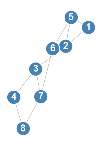
Figure 3.3: A graph with three connected components.
Now we can check that there are exactly 3 zero eigenvalues.
L = laplacian(G)eigvals, eigvecs = np.linalg.eig(L)num_0_eigs = np.isclose(eigvals, 0, atol =1e-10).sum() # number of zero eigenvaluesprint("Number of zero eigenvalues: ", num_0_eigs)
Number of zero eigenvalues: 3
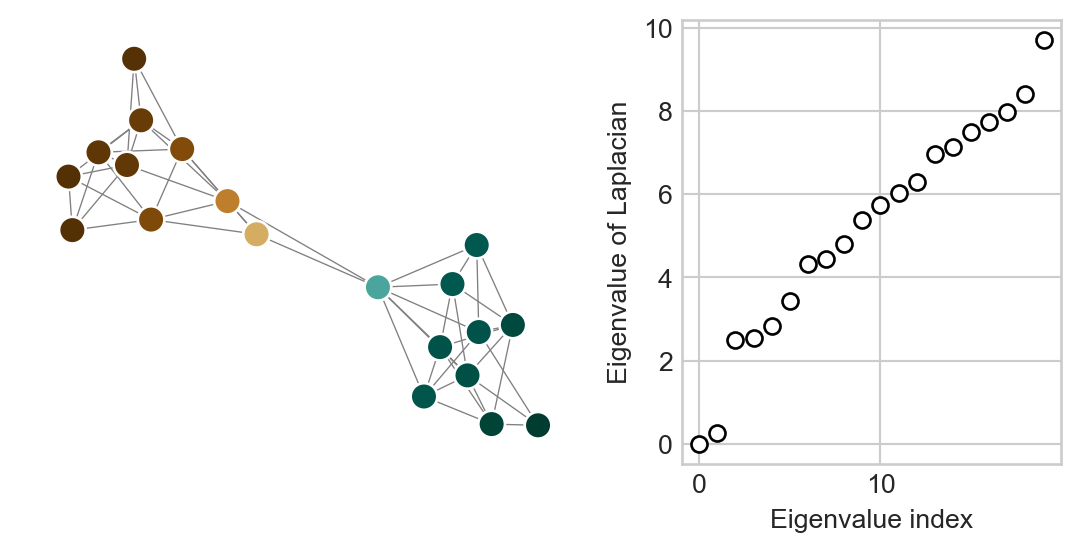
In a graph with just one connected component, Theorem 3.5 implies that there is exactly one zero eigenvalue of \(\mathbf{L}\). It turns out that if the graph is “almost disconnected” into two components, then the second-smallest eigenvalue of the Laplacian will be “almost 0”. This is part of the motivation behind Laplacian spectral clustering, an algorithm which we’ll see later on. Here’s an example of such a graph, which we’ve plotted alongside the eigenvalues of the Laplacian:
This kind of structure is often called community structure and we will study it much more later in the course.
Figure 3.4: (Left) A graph which is almost disconnected into two components; deleting two edges would separate the network. (Right): the eigenvalues of the Laplacian of the graph in ascending order. The second-smallest eigenvalue is very close to 0, which reflects the near-disconnectedness of the graph. Nodes in the graph are colored according to the corresponding eigenvector
The eigenvalue on the very far left is the zero eigenvalue guaranteed for any graph, while the very small eigenvalue right next to it reflects the structure of the graph as “almost disconnected” into two components.
The Graph Laplacian as a Smoothness Measure
Suppose that we have a vector \(\mathbf{x} \in \mathbb{R}^n\), where we interpret entry \(x_i\) as describing some quantity at node \(i\). The Laplacian matrix can be used to measure the “smoothness” of this vector on the graph, by which we mean the extent to which neighboring nodes have similar values of \(x\). One way to quantify this is using the measure
The term corresponding to \(i\) and \(j\) in \(S(\mathbf{x})\) is zero if either \(A_{ij} = 0\) (i.e. node \(i\) is not connected to node \(j\)) or if \(x_i = x_j\) (i.e. nodes \(i\) and \(j\) have the same values in their corresponding entries of \(\mathbf{x}\)). So, intuitively, \(S(\mathbf{x})\) is small when connected nodes have similar entries in \(\mathbf{x}\) and large when connected nodes have very different entries in \(\mathbf{x}\). The Laplacian can be used to concisely represent the smoothness measure \(S(\mathbf{x})\):
In the last line, we’ve used the definition of the degree: \(k_i = \sum_{j = 1}^n A_{ij}\). Now we need to use an indexing trick. Let \(\delta_{ij}\) be the Kronecker delta, which is 1 if \(i = j\) and 0 otherwise. Then, we can write
So, our smoothness measure is the quadratic form \(\mathbf{x}^T\mathbf{Lx}\). The role of the Laplacian in measuring the smoothness of functions defined on graphs is another perspective on its use in both algorithms and modeling of dynamical systems.
To operationalize this, let’s implement a smoothness score:
Show code
def smoothness(G, x): L = laplacian(G)return x@L@x
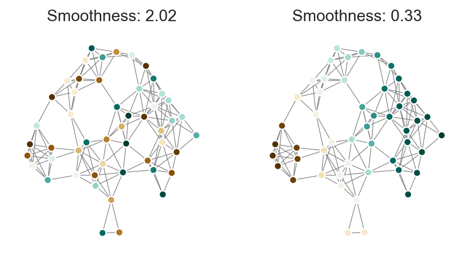
Now we can compare the smoothness of a random vector with the smoothness of a vector that varies in a more continuous fashion across the graph. I’ve obtained the smooth vector as the eigenvector corresponding to the second-smallest eigenvalue (as in the example above), but this isn’t important in this context; it’s just one convenient way to get a smooth vector.
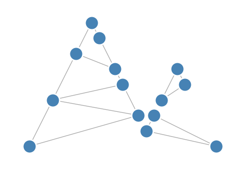
Figure 3.5: Two functions defined on the nodes of a graph and their corresponding smoothness scores as measured by the Laplacian.
Indeed, the vector which varies more smoothly across the graph (with fewer large large “jumps” along edges) has a much smaller smoothness score.
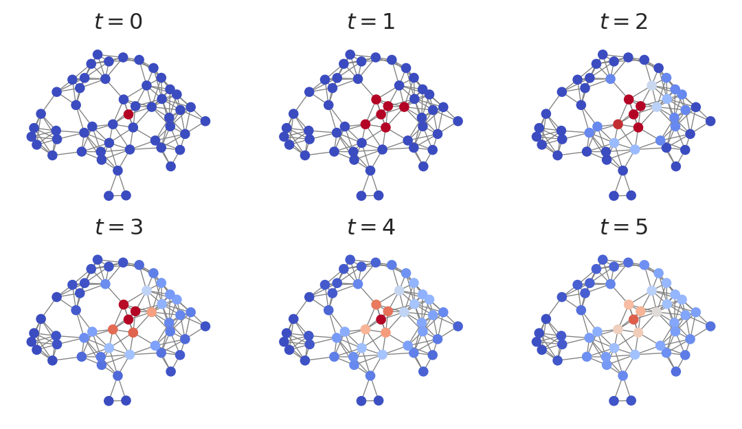
The Graph Laplacian as a Diffusion Operator
One of the many important properties of the graph Laplacian is that it describes many spreading or diffusion processes that take place on networks. Here’s an example: suppose that we “heat up” a single node on the network, and then allow heat to flow along the network edges. The Laplacian matrix gives a concise description of how this heat spreads over the network. Let \(\mathbf{x} \in \mathbb{R}^n\) be the vector whose \(i\)th entry gives the amount of heat currently on node \(i\). Then, the vector \(\delta \mathbf{x} = -\mathbf{Lx}\) is proportional to rate of change of heat at each node. If we imagine that heat moves in discrete time, our update would be
One perspective on this update is that it is the gradient flow associated with minimization of the smoothness measure \(S(\mathbf{x})\) from the previous section.