10 Preferential Attachment and Power Laws

Open the live notebook in Google Colab here.

In a previous chapter, we discussed several properties observed in empirical networks. One of the properties we observed was an (approximate) power law degree distribution. It has been famously claimed (Barabási and Albert 1999) that many empirical networks have power-law degrees, a claim which has also been famously disputed(Broido and Clauset 2019).

We’re not going to take a stance on the question of whether many empirical networks obey power laws in this chapter. Instead, we’ll focus on a modeling question: if we supposed that power laws are present in many real-world systems, how could we explain that? One way to address this question is via mathematical modeling: can we come up with a plausible mathematical model of networks that would reliably generate power-law degree distributions? There have been a number of such models proposed; in these notes we’ll discuss a variation on one of the most famous; the Yule-Simon-Price-Barabási-Albert model of preferential attachment.

This model was made famous by Barabási and Albert (1999), but their model is very similar to the regrettably much less famous models of Yule (1925), Simon (1955), and Price (1976)

To motivate our discussion, let’s take another look at a network which displays an approximate power law degree distribution. We’ll again use the twitch data set collected from the streaming platform Twitch by Rozemberczki, Allen, and Sarkar (2021). Nodes are users on Twitch. An edge exists between them if they are mutual friends on the platform. The authors collected data sets for users speaking several different languages; we’ll use the network of English-speaking users. Let’s now download the data (as a Pandas data frame) and convert it into a graph using Networkx.

The hidden code block contains package imports and plotting style configuration.

Show code

from matplotlib import pyplot as plt
import networkx as nx
plt.style.use('seaborn-v0_8-whitegrid')
import numpy as np
from scipy.special import factorial
import pandas as pd
import random

url = "https://raw.githubusercontent.com/benedekrozemberczki/MUSAE/master/input/edges/ENGB_edges.csv"
edges = pd.read_csv(url)
G = nx.from_pandas_edgelist(edges, "from", "to", create_using=nx.Graph)

num_nodes = G.number_of_nodes()
num_edges = G.number_of_edges()

print(f"This graph has {num_nodes} nodes and {num_edges} edges. The mean degree is {2*num_edges/num_nodes:.1f}.")

This graph has 7126 nodes and 35324 edges. The mean degree is 9.9.

We’ll use the same helper functions for visualizing the degree distribution as a log-binned histogram as we used previously, implemented in the hidden code cell below.

Show code

def degree_sequence(G):
    degrees = nx.degree(G)
    degree_sequence = np.array([deg[1] for deg in degrees])
    return degree_sequence

def log_binned_histogram(degree_sequence, interval = 5, num_bins = 20):
    hist, bins = np.histogram(degree_sequence, bins = min(int(len(degree_sequence)/interval), num_bins))
    bins = np.logspace(np.log10(bins[0]),np.log10(bins[-1]),len(bins))
    hist, bins = np.histogram(degree_sequence, bins = bins)
    binwidths = bins[1:] - bins[:-1]
    hist = hist / binwidths
    p = hist/hist.sum()

    return bins[:-1], p

def plot_degree_distribution(G, **kwargs):

    deg_seq = degree_sequence(G)
    x, p = log_binned_histogram(deg_seq, **kwargs)
    plt.scatter(x, p,  facecolors='none', edgecolors =  'cornflowerblue', linewidth = 2, label = "Data")
    plt.gca().set(xlabel = "Degree", xlim = (0.5, x.max()*2))
    plt.gca().set(ylabel = "Density")
    plt.gca().loglog()
    plt.legend()
    return plt.gca()

Let’s use this function to inspect the degree distribution of the data:

ax = plot_degree_distribution(G, interval = 10, num_bins = 30)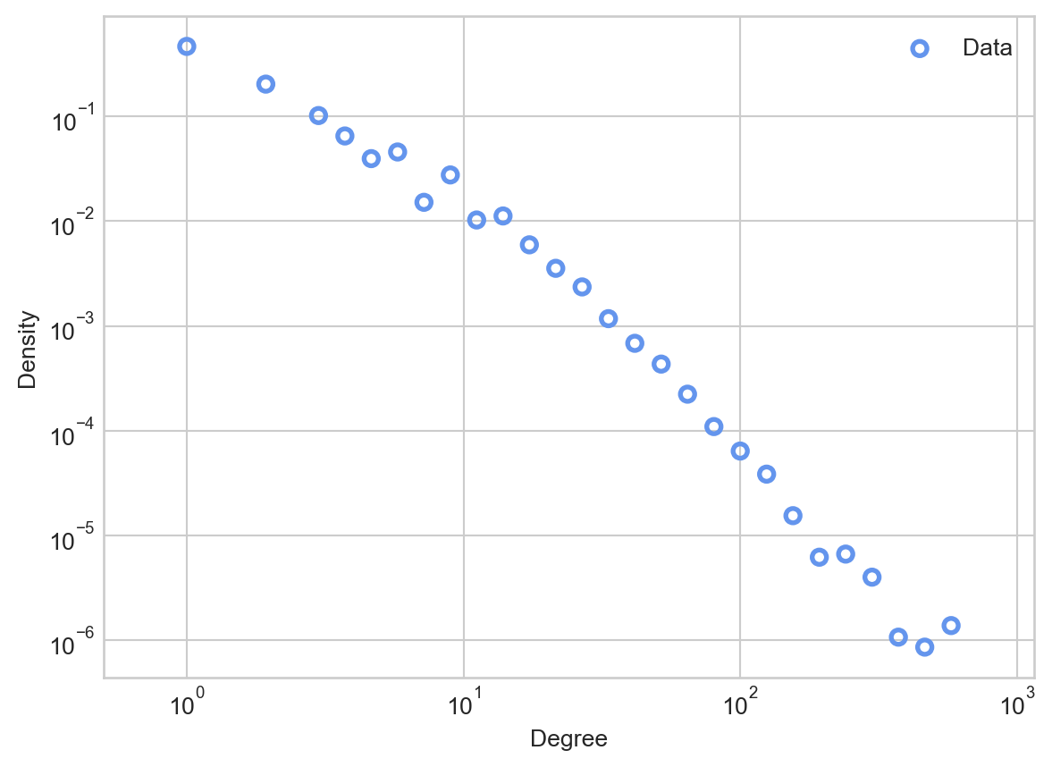

There are a few things to notice about this degree distribution. First, most nodes have relatively small degrees, fewer than the mean of 9.9. However, there are a small number of nodes that have degrees which are much larger: almost two orders of magnitude larger! You can think of these nodes as “super stars” or “hubs” of the network; they may correspond to especially popular or influential accounts.

Recall that, from our discussion of the Erdős–Rényi model $G (n, p)$ , the degree distribution of a $G (n, p)$ model with mean degree $\bar{k}$ is approximately Poisson with mean $\bar{k}$ . Let’s compare this Poisson distribution to the data.

deg_seq = degree_sequence(G)
mean_degree  = deg_seq.mean()
d_      = np.arange(1, 30, 1)
poisson = np.exp(-mean_degree)*(mean_degree**d_)/factorial(d_)

ax = plot_degree_distribution(G, interval = 10, num_bins = 30)
ax.plot(d_, poisson,  linewidth = 1, label = "Poisson fit", color = "grey", linestyle = "--")
ax.legend()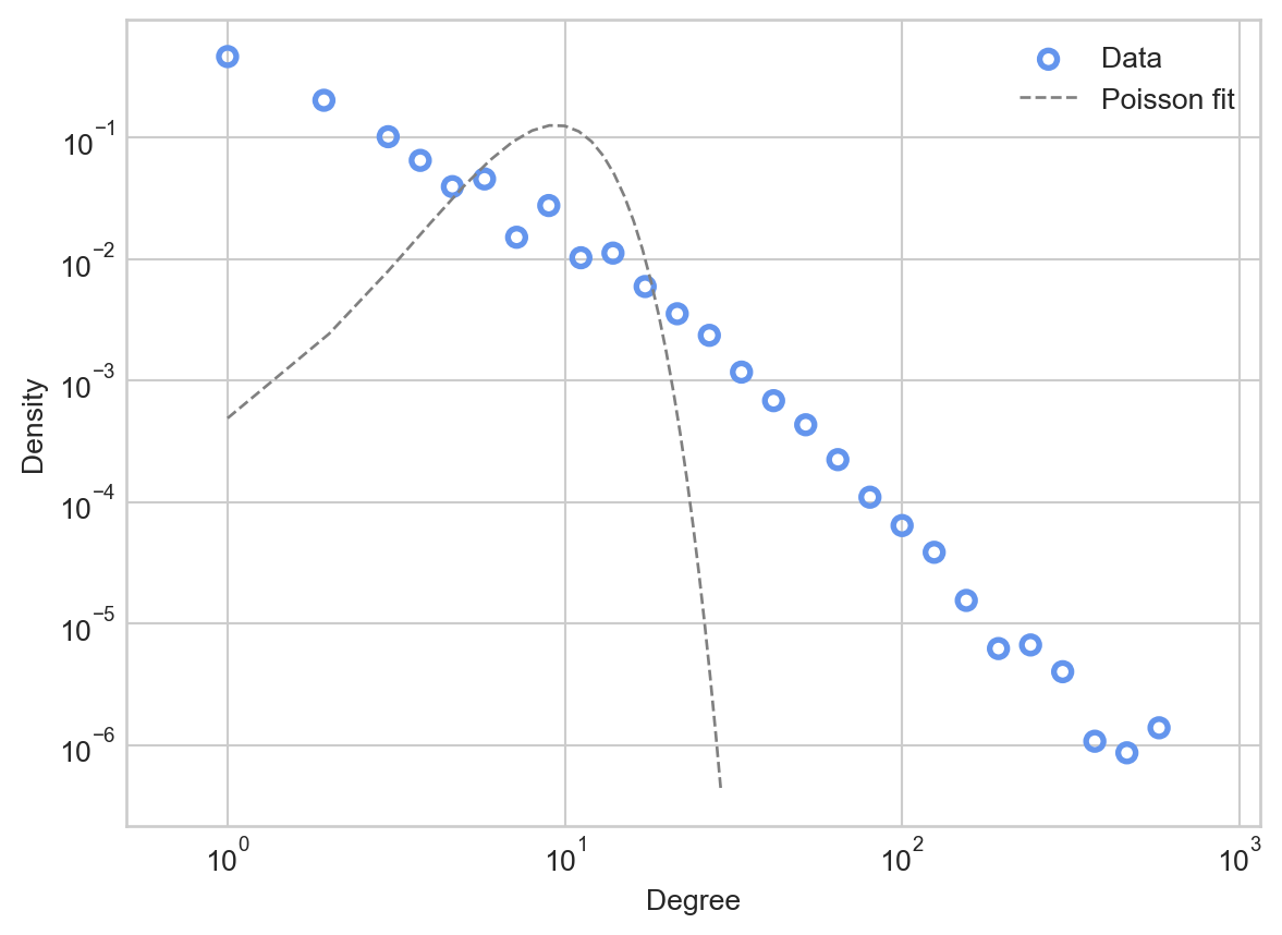

Comparing the Poisson fit predicted by the Erdős–Rényi model to the actual data, we see that the the Poisson places much higher probability mass on degrees that are close to the mean of 9.9. The Poisson would predict that almost no nodes would have degree higher than $10^{2}$ , while in the data there are several.

We often say that the Poisson has a “light right tail” – the probability mass allocated by the Poisson dramatically drops off as we move to the right of the mean. In contrast, the data itself appears to have a “heavy tail”: there is substantial probability mass even far to the right from the mean.

Recap: Power Laws

Definition 10.1 (Power Law Distribution) A random variable $K$ has a discrete power law distribution with cutoff $k_{*}$ and exponent $γ > 1$ if its probability mass function is has the form

$\begin{matrix} (10.1) & \begin{array}{r} p_{k} ≜ P [K = k] = C k^{- γ}, \end{array} \end{matrix}$

for all $k > k_{*}$ . Here, $C$ is a normalizing constant that ensures that the distribution sums to $1$ . The entries of the distribution for $k \leq k_{*}$ are are arbitrary provided that the entire probability distribution normalizes.

As we saw previously, power law distributions are linear when plotted on log-log axes. The expectation of a power-law distributed random variable is finite when $γ > 2$ and the variance is finite when $γ > 3$ .

Let’s try plotting such a distribution against the data. Since the power law distribution is defined for all $k > k_{*}$ , we’ll need to choose a cutoff $k_{*}$ and an exponent $γ$ . For now, we’ll do this by eye. If we inspect the plot of the data above, it looks like linear behavior takes over somewhere around $k_{*} = 10^{\frac{3}{2}} \approx 30$ .

deg_seq = degree_sequence(G)
cutoff  = 30
d_      = np.arange(cutoff, deg_seq.max(), 1)
gamma   = 2.7
power_law = 18*d_**(-gamma)

ax = plot_degree_distribution(G, interval = 10, num_bins = 30)
ax.plot(d_, power_law,  linewidth = 1, label = fr"Power law: $\gamma = {gamma}$" , color = "grey", linestyle = "--")
ax.legend()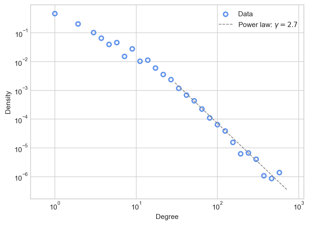

The power law appears to be a much better fit than the Poisson to the tail of the distribution, making apparently reasonable predictions about the numbers of nodes with very high degrees.

Where do the parameters for the power law come from? Here we performed a fit “by eye”, but we discuss some systematic approaches in Section 10.4

The claim that a given network “follows a power law” is a bit murky: like other models, power laws are idealizations that no real data set matches exactly. The idea of a power law is also fundamentally asymptotic in nature: the power law that we fit to the data also predicts that we should see nodes of degree $10^{3}$ , $10^{4}$ , or $10^{5}$ if we were to allow the network to keep growing. Since the network can’t keep growing (it’s data, we have a finite amount of it), we have to view the power law’s predictions about very high-degree nodes as extrapolations toward an idealized, infinite-size data set to which we obviously do not have access.

The Preferential Attachment Model: A Generative Model for Power Law Degrees

Why would power-law degree distributions be common in empirical networks? A common way to answer questions like this is to propose a generative model. A generative model is a random network model that is intended to produce some kind of realistic structure. If the mechanism proposed by the generative model is plausible as a real, common mechanism, then we might expect that the large-scale structure generated by that model would be commonly observed.

Generative models contrast with null models like the

G (n, p)

model, which are usually used to contrast with real networks. Generative models are models of what the data is like; null models are models of what the data is not like.

Barabási and Albert (1999) are responsible for popularizing the claim that many empirical networks are scale-free. Alongside this claim, they offered a generative model called preferential attachment. The preferential attachment model offers a simple mechanism of network growth which leads to power-law degree distributions. Their model is closely related to the regrettably much less famous models of Yule (1925), Simon (1955), and Price (1976).

Here’s how the Yule-Simon-Price-Barabási-Albert model works. First, we start off with some initial graph $G_{0}$ . Then, in each timestep $t = 1, 2, \dots$ , we:

The model of Barabási and Albert (1999) did not include a uniform selection mechanism, which corresponds to the case

α = 1

Flip a coin with probability of heads equal to $α$ . If this coin lands heads, then:
1. Choose a node $u$ from $G_{t - 1}$ with probability proportional to its degree.
Otherwise, if the coin lands tails, choose a node $u$ from $G_{t - 1}$ uniformly at random.
Add a node $v$ to $G_{t - 1}$ .
Add edge $(u, v)$ to $G_{t - 1}$ .

We repeat this process as many times as desired. Intuitively, the preferential attachment model expresses the idea that “the rich get richer”: nodes that already have many connections are more likely to receive new connections.

Here’s a quick implementation.

Note: this implementation of preferential attachment is useful for illustrating the mathematics and operations with Networkx. It is, however, not efficient.

# initial condition
G = nx.Graph() 
G.add_edge(0, 1) 

alpha = 4/5 # proportion of degree-based selection steps

# main loop
for _ in range(10000):
    degrees = nx.degree(G)

    # determine u using one of two mechanisms
    if np.random.rand() < alpha: 
        deg_seq = np.array([deg[1] for deg in degrees])
        degree_weights = deg_seq / deg_seq.sum()
        u = np.random.choice(np.arange(len(degrees)), p = degree_weights)
    else: 
        u = np.random.choice(np.arange(len(degrees)))

    # integer index of new node v
    v = len(degrees)

    # add new edge to graph    
    G.add_edge(u, v)

Let’s go ahead and plot the result. We’ll add a visualization of the exponent $γ$ as well. How do we know the right value of $γ$ ? It turns out that there is a theoretical estimate based on $α$ which we’ll derive in the next section.

deg_seq = degree_sequence(G)
cutoff  = 10
d_      = np.arange(cutoff, deg_seq.max(), 1)
gamma   = (2 + alpha) / alpha
power_law = 10*d_**(-gamma)

ax = plot_degree_distribution(G, interval = 2, num_bins = 30)
ax.plot(d_, power_law,  linewidth = 1, label = fr"Power law: $\gamma = {gamma:.2f}$" , color = "grey", linestyle = "--")
ax.legend()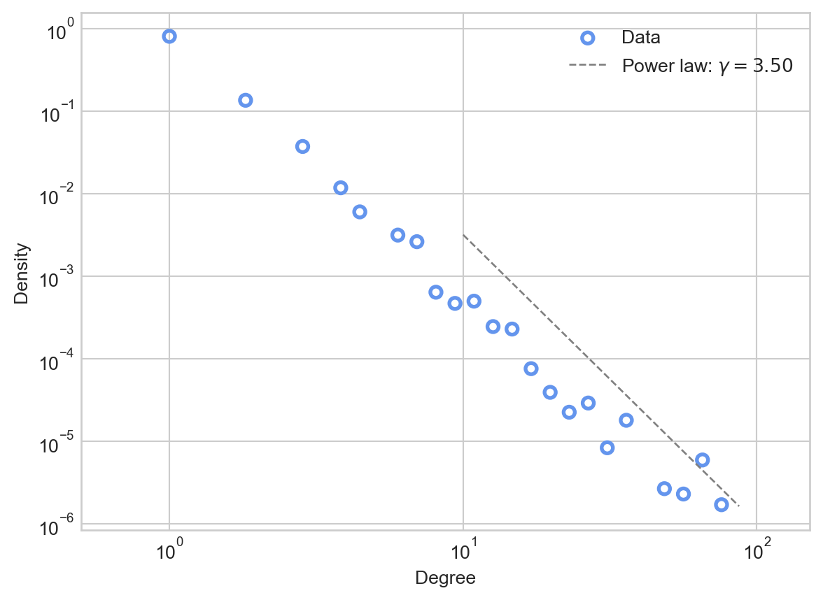

This fit is somewhat noisy, reflecting the fact that we simulated a relatively small number of preferential attachment steps.

Analyzing Preferential Attachment

Let’s now see if we can understand mathematically why the preferential attachment model leads to networks with power-law degree distributions. There are many ways to demonstrate this fact, including both “casual” and highly rigorous techniques. Here, we’ll use a “casual” argument from Mitzenmacher (2004).

Let $p_{k}^{(t)}$ be the proportion of nodes of degree $k \geq 2$ after algorithmic timestep $t$ . Suppose that at this timestep there are $n$ nodes and $m$ edges. Then, the total number of nodes of degree $d$ is $n_{k}^{(t)} = n p_{k}^{(t)}$ . Suppose that we do one step of the preferential attachment model. Let’s ask: what will be the new expected value of $n_{k}^{(t + 1)}$ ?

Well, in the previous timestep there were $n_{k}^{(t)}$ nodes of degree $k$ . How could this quantity change? There are two processes that could make $n_{k}^{(t + 1)}$ different from $n_{k}^{(t)}$ . If we selected a node $u$ with degree $k - 1$ in the model update, then this node will become a node of degree $k$ (since it will have one new edge attached to it), and will newly count towards the total $n_{k}^{(t + 1)}$ . On the other hand, if we select a node $u$ of degree $k$ , then this node will become a node of degree $k + 1$ , and therefore no longer count for $n_{k}^{(t + 1)}$ .

So, we can write down our estimate for the expected value of $n_{k}^{(t + 1)}$ .

$\begin{array}{r} E [n_{k}^{(t + 1)}] - n_{k}^{(t)} = P [k_{u} = k - 1] - P [k_{u} = k] . \end{array}$

Let’s compute the probabilities appearing on the righthand side. With probability $α$ , we select a node from $G_{t}$ proportional to its degree. This means that, if a specific node $u$ has degree $k - 1$ , the probability of picking $u$ is

$\begin{array}{r} P [u is picked] = \frac{k - 1}{\sum_{w \in G} k_{w}} = \frac{k - 1}{2 m^{(t)}} . \end{array}$

Of all the nodes we could pick, $p_{k - 1}^{(t)} n$ of them have degree $k - 1$ . So, the probability of picking a node with degree $k - 1$ is $n p_{k - 1}^{(t)} \frac{k - 1}{2 m}$ . On the other hand, if we flipped a tails (with probability $1 - α$ ), then we pick a node uniformly at random; each one is equally probable and $p_{k - 1}^{(t)}$ of them have degree $k - 1$ . So, in this case the probability is simply $p_{k - 1}^{(t)}$ . Combining using the law of total probability, we have

$\begin{aligned} P [k_{u} = k - 1] & = α n p_{k - 1}^{(t)} \frac{k - 1}{2 m^{(t)}} + (1 - α) p_{k - 1}^{(t)} \\ = [α n \frac{k - 1}{2 m} + (1 - α)] p_{k - 1}^{(t)} . \end{aligned}$

A similar calculation shows that

$\begin{aligned} P [k_{u} = k] & = α n p_{k}^{(t)} \frac{k}{2 m^{(t)}} + (1 - α) p_{k}^{(t)} \\ = [α n \frac{k}{2 m} + (1 - α)] p_{k}^{(t)}, \end{aligned}$

so our expectation is

$\begin{array}{r} E [n_{k}^{(t + 1)}] - n_{k}^{(t)} = [α n \frac{k - 1}{2 m} + (1 - α)] p_{k - 1}^{(t)} - [α n \frac{k}{2 m} + (1 - α)] p_{k}^{(t)} . \end{array}$

Up until now, everything has been exact: no approximations involved. Now we’re going to start making approximations and assumptions. These can all be justified by rigorous probabilistic arguments, but we won’t do this here.

We’ll assume that $n_{k}^{(t + 1)}$ is equal to its expectation.
In each timestep, we add one new node and one new edge. This means that, after enough timesteps, the number of nodes $n$ and number of edges $m$ should be approximately equal. We’ll therefore assume that $t$ is sufficiently large that $\frac{n}{m} \approx 1$ .
Stationarity: we’ll assume that, for sufficiently large $t$ , $p_{k}^{(t)}$ is a constant: $p_{k}^{(t)} = p_{k}^{(t + 1)} ≜ p_{k}$ .

To track these assumptions, we’ll use the symbol $≐$ to mean “equal under these assumptions.”

With these assumptions, we can simplify. First, we’ll replace $E [n_{k}^{(t + 1)}]$ with $n_{k}^{(t + 1)}$ , which we’ll write as $(n + 1) p_{k}^{(t + 1)}$

$\begin{array}{r} (n + 1) p_{k}^{(t + 1)} - n p_{k}^{(t)} ≐ [α n \frac{k - 1}{2 m} + (1 - α)] p_{k - 1}^{(t)} - [α n \frac{k}{2 m} + (1 - α)] p_{k}^{(t)} . \end{array}$

Next, we’ll assume $\frac{n}{m} \approx 1$ :

$\begin{array}{r} (n + 1) p_{k}^{(t + 1)} - n p_{k}^{(t)} ≐ [α \frac{k - 1}{2} + (1 - α)] p_{k - 1}^{(t)} - [α \frac{k}{2} + (1 - α)] p_{k}^{(t)} . \end{array}$

Finally, we’ll assume stationarity:

$\begin{array}{r} (n + 1) p_{k} - n p_{k} ≐ [α \frac{k - 1}{2} + (1 - α)] p_{k - 1} - [α \frac{k}{2} + (1 - α)] p_{k} . \end{array}$

After a long setup, this looks much more manageable! Our next step is to solve for $p_{k}$ , from which we find

$\begin{aligned} p_{k} & ≐ \frac{α \frac{k - 1}{2} + (1 - α)}{1 + α \frac{k}{2} + (1 - α)} p_{k - 1} \\ = \frac{2 (1 - α) + (k - 1) α}{2 (1 - α) + 2 + k α} p_{k - 1} \\ = (1 - \frac{2 + α}{2 (1 - α) + 2 + k α}) p_{k - 1} . \end{aligned}$ When $k$ grows large, this expression is approximately $\begin{array}{r} p_{k} ≃ (1 - \frac{1}{k} \frac{2 + α}{α}) p_{k - 1} . \end{array}$

Now for a trick “out of thin air.” As $k$ grows large,

$\begin{array}{r} 1 - \frac{1}{k} \frac{2 + α}{α} \to {(\frac{k - 1}{k})}^{\frac{2 + α}{α}} \end{array}$

Exercise

Justify the approximation above. To do this, Taylor-expand the function $f (x) = x^{γ}$ to first order around the point $x_{0} = 1$ and use this expansion to estimate the value of $1 - \frac{1}{k}$ .

Applying this last approximation, we have shown that, for sufficiently large $k$ ,

$\begin{array}{r} p_{k} ≃ {(\frac{k - 1}{k})}^{\frac{2 + α}{α}} p_{k - 1} . \end{array}$

This recurrence relation, if it were exact, would imply that $p_{k} = C d^{- \frac{2 + α}{α}}$ , as shown by the following exercise:

Exercise

Suppose that $p_{k}$ is a probability distribution with the property that, for some $k_{*}$ and for all $d > k_{*}$ , it holds that

$\begin{array}{r} p_{k} = {(\frac{k - 1}{k})}^{γ} p_{k - 1} . \end{array}$

Prove using induction that $p_{k} = C k^{- γ}$ for some constant $C$ , and explain how to compute $C$ .

This concludes our argument. Although this argument contains many approximations, it is also possible to reach the same conclusion using fully rigorous probabilistic arguments (Bollobás et al. 2001).

We’ve shown that, when $k$ is large and in approximation,

$\begin{array}{r} p_{k} = C d^{- \frac{2 + α}{α}}, \end{array}$

which is a power law with $γ = \frac{2 + α}{α}$ . This means that the smallest value of $γ$ we can achieve is $γ = 3$ . Many estimates of the value of $γ$ in empirical networks are close to 3, although some are smaller (and therefore not able to be produced by this version of the preferential attachment model).

Estimating Power Laws From Data

After the publication of Barabási and Albert (1999), there was a proliferation of papers purporting to find power-law degree distributions in empirical networks. For a time, the standard method for estimating the exponent $γ$ was to use the key visual signature of power laws – power laws are linear on log-log axes. This suggests performing linear regression in log-log space; the slope of the regression line is the estimate of $γ$ . This approach, however, is badly flawed: errors can be large, and uncertainty quantification is not reliably available. Clauset, Shalizi, and Newman (2009) discuss this problem in greater detail, and propose an alternative scheme based on maximum likelihood estimation and goodness-of-fit tests. Although the exact maximum-likelihood estimate of $γ$ is the output of a maximization problem and is not available in closed form, the authors supply a relatively accurate approximation:

$\begin{array}{r} \hat{γ} = 1 + n {(\sum_{i = 1}^{n} \log \frac{k_{i}}{k_{*}})}^{- 1} . \end{array}$

As they show, this estimate and related methods are much more reliable estimators of $γ$ than the linear regression method.

An important cautionary note: the estimate $\hat{γ}$ can be formed regardless of whether or not the power law is a good descriptor of the data. Supplementary methods such as goodness-of-fit tests are necessary to determine whether a power law is appropriate at all. Clauset, Shalizi, and Newman (2009) give some guidance on such methods as well.

Preferential Attachment in Growing Graphs

What if we are able to observe more than the degree distribution of a network? What if we could also observe the growth of the network, and actually know which edges were added at which times? Under such circumstances, it is possible to estimate more directly the extent to which a graph might grow via the preferential attachment mechanism, possibly alongside additional mechanisms. Overgoor, Benson, and Ugander (2019) supply details on how to estimate the parameters of a general class of models, including preferential attachment, from observed network growth.

Are Power Laws Good Descriptors of Real-World Networks?

Are power laws really that common in empirical data? Broido and Clauset (2019) controversially claimed that scale free networks are rare. In a bit more detail, the authors compare power-law distributions to several competing distributions as models of real-world network degree sequences. The authors find that that the competing models—especially lognormal distributions, which also have heavy tails—are often better fits to observed data than power laws. This paper stirred considerable controversy, which is briefly documented by Holme (2019).

References

Barabási, Albert-László, and Réka Albert. 1999. “Emergence of Scaling in Random Networks.” Science 286 (5439): 509–12. https://doi.org/10.1126/science.286.5439.509.

Bollobás, Bela, Oliver Riordan, Joel Spencer, and Gábor Tusnády. 2001. “The Degree Sequence of a Scale-Free Random Graph Process.” Random Structures & Algorithms 18 (3): 279–90. https://doi.org/10.1002/rsa.1009.

Broido, Anna D., and Aaron Clauset. 2019. “Scale-Free Networks Are Rare.” Nature Communications 10 (1): 1017. https://doi.org/10.1038/s41467-019-08746-5.

Clauset, Aaron, Cosma Rohilla Shalizi, and Mark E. J. Newman. 2009. “Power-Law Distributions in Empirical Data.” SIAM Review 51 (4): 661–703. https://doi.org/10.1137/070710111.

Holme, Petter. 2019. “Rare and Everywhere: Perspectives on Scale-Free Networks.” Nature Communications 10 (1): 1016. https://doi.org/10.1038/s41467-019-09038-8.

Mitzenmacher, Michael. 2004. “A Brief History of Generative Models for Power Law and Lognormal Distributions.” Internet Mathematics 1 (2): 226–51. https://doi.org/10.1080/15427951.2004.10129088.

Overgoor, Jan, Austin Benson, and Johan Ugander. 2019. “Choosing to Grow a Graph: Modeling Network Formation as Discrete Choice.” In The World Wide Web Conference, 1409–20. San Francisco CA USA: ACM. https://doi.org/10.1145/3308558.3313662.

Price, Derek de Solla. 1976. “A General Theory of Bibliometric and Other Cumulative Advantage Processes.” Journal of the American Society for Information Science 27 (5): 292–306.

Rozemberczki, Benedek, Carl Allen, and Rik Sarkar. 2021. “Multi-Scale Attributed Node Embedding.” Journal of Complex Networks 9 (2).

Simon, Herbert A. 1955. “On a Class of Skew Distribution Functions.” Biometrika 42 (3-4): 425–40. https://doi.org/10.1093/biomet/42.3-4.425.

Yule. 1925. “A Mathematical Theory of Evolution, Based on the Conclusions of Dr. J. C. Willis, F. R. S.” Philosophical Transactions of the Royal Society of London. Series B, Containing Papers of a Biological Character 213 (402-410): 21–87. https://doi.org/10.1098/rstb.1925.0002.