Show code
import networkx as nx
import numpy as np
from itertools import combinations
from matplotlib import pyplot as plt
plt.style.use('seaborn-v0_8-whitegrid')

np.random.seed(1234)Open the live notebook in Google Colab here.
Recently, we measured several properties of real-world networks. Some of our measurements included the number of connected components, the proportion of possible triangles realized, and the mean length of paths between nodes. When interpreting these measurements, we face two important questions:
- Is a given observation of an empirical network interesting or surprising in some way?
- What properties of the graph would be sufficient to explain that observation?
For example, suppose that we measure the transitivity (proportion of realized triangles) in a graph and find a value of \(0.4\). Is that interesting or surprising? If so, how would we explain it? For example, would the degree sequence alone be sufficient to explain this observation, or would we need to consider more detailed graph properties in order to explain it?
The way that we usually approach these questions is with mathematical models of graphs. We determine whether measurements are surprising by comparing to mathematical models. We can also design models that hold certain features fixed (like the degree sequence) in order to see whether those features are sufficient on their own to explain the value of other measurements (like transitivity). Because real data is usually messy and noisy, it’s helpful for us to allow our mathematical models to be messy and noisy too! Our models are therefore random models of graphs, or just random graphs for short.
In addition to the role of random graphs in contextualizing and explaining network measurements, they are also very interesting mathematical objectis in their own right! Indeed, there is an entire field of mathematics about the theory of random graphs. Random graph models are also helpful for algorithms for network data analysis, including in both the design and analysis of these algorithms.
The model of Erdős and Rényi (1960) is the simplest and most fundamental model of a random graph. Our primary interest in the ER model is for mathematical insight and null modeling. The ER model is mostly understood in its major mathematical properties, and it’s almost never used in statistical inference.
We can imagine visiting each possible pair of edges \((i,j)\) and flipping an independent coin with probability of heads \(p\). If heads, we add \((i,j) \in E\); otherwise, we don’t. Indeed, one (relatively inefficient) implementation of the \(G(n,p)\) model works exactly like this.
import networkx as nx
import numpy as np
from itertools import combinations
from matplotlib import pyplot as plt
plt.style.use('seaborn-v0_8-whitegrid')
np.random.seed(1234)def gnp(n, p):
G = nx.Graph()
for i, j in combinations(range(n), 2): # all pairs of nodes
if np.random.rand() < p:
G.add_edge(i, j)
return GHaving implemented this function, we can now generate a graph.
G = gnp(100, 0.03)nx.draw(G,
node_size = 100,
edge_color = "gray",
width = 0.5,
edgecolors = "white",
node_color = "steelblue")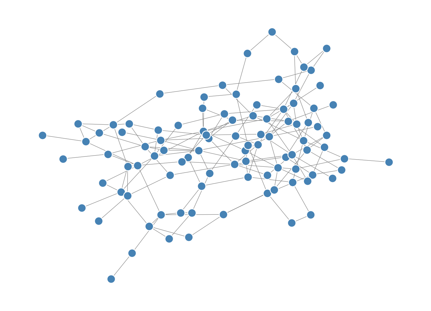
This approach to generating \(G(n,p)\) graphs by looping through all pairs of edges is not the most efficient possible; see Ramani, Eikmeier, and Gleich (2019) for faster algorithms.
Let’s now explore some of the fundamental mathematical properties of \(G(n,p)\) graphs.
Let’s work an example of estimating a property of the \(G(n,p)\) model. We’re going to estimate the transitivity, also called the global clustering coefficient of the \(G(n,p)\) model. Recall that the transitivity is defined as
\[ \begin{aligned} T = \frac{\text{number of triangles}}{\text{number of wedges}}\;. \end{aligned} \]
Here, a wedge on node \(i\) is a possible triangle: two edges \((i,j)\) and \((i,k)\). The addition of the edge \((j,k)\) would complete the triangle.
Let’s estimate the value of \(T\) for the \(G(n,p)\) model. Analyzing ratios using probability theory can get tricky, but we can get a pretty reliable picture of things by computing the expectations of the numerator and denominator separately.
How many triangles are there? We can choose a “base” node \(i\) in \(n\) ways and then choose a pair of additional nodes \(j\) and \(k\) in \(\binom{n-1}{2}\) ways. The probability that all three edges exist is \(p^3\). So, in expectation, there are \(n\binom{n-1}{2}p^3\) triangles in the graph.
On the other hand, how many wedges are there? We can again choose the base node \(i\) and the two additional nodes in a total of \(n\binom{n-1}{2}\) ways. A wedge (potential triangle) exists if the edges \((i,j)\) and \((i,k)\) are present, which occurs with probability \(p^2\).
The ratio between these two expectations is \(p\). Indeed, it’s possible to prove using concentration inequalities that, in this case, the expected transitivity is indeed very close to this ratio of expectations.
Let’s compute the transitivity of a \(G(n,p)\) graph with NetworkX. We’ll use a larger graph size for this experiment:
G = nx.fast_gnp_random_graph(1000, 0.03)
nx.transitivity(G)0.029832725995521798The observed value of the clustering coefficient is close to the prediction of our approximate calculation.
Recall that it is possible to define sparsity more explicitly when we have a theoretical model (where it makes sense to take limits). Indeed, the sparse Erdős–Rényi model is very useful. Intuitively, the idea of sparsity is that there are not very many edges in comparison to the number of nodes.
A consequence of sparsity is that \(\mathbb{E}[K_i] = c\); i.e. the expected degree of a node in sparse \(G(n,p)\) is constant. When studying sparse \(G(n,p)\), we are almost always interested in reasoning in the limit \(n\rightarrow \infty\).
It is possible to show that, when \(p = c/(n-1)\), the degree of a node in sparse \(G(n,p)\) converges (in distribution) to a Poisson random variable with mean \(c\). For this reason, the \(G(n,p)\) is also sometimes called the Poisson random graph.
What does this imply for our estimation of the global clustering coefficient from before? Well, we expect the global clustering coefficient to be about \(p\), and if \(p = c/(n-1)\), then \(p \rightarrow 0\) as \(n \to \infty\) for sparse \(G(n,p)\). We’ve given a heuristic argument showing that \(T \approx p\), and so our analysis predicts:
Sparse Erdős–Rényi graphs have vanishing clustering coefficients.
Figure 7.2 shows how the global clustering coefficient of a sparse Erdős–Rényi random graph decays as we increase \(n\).
c = 5
N = np.repeat(2**np.arange(5, 15), 10)

def global_clustering(n, c):
    G = nx.fast_gnp_random_graph(n, c/(n-1))
    return nx.transitivity(G)

T = [global_clustering(n, c) for n in N]

fig, ax = plt.subplots(1)

theory = ax.plot(N, c/(N-1), color = "black", label = "Estimate")

exp = ax.scatter(N, T, label = "Experiments", color = "steelblue", s = 10)
semil = ax.loglog()
labels = ax.set(xlabel = "Number of nodes",
       ylabel = "Global clustering coefficient")
plt.show()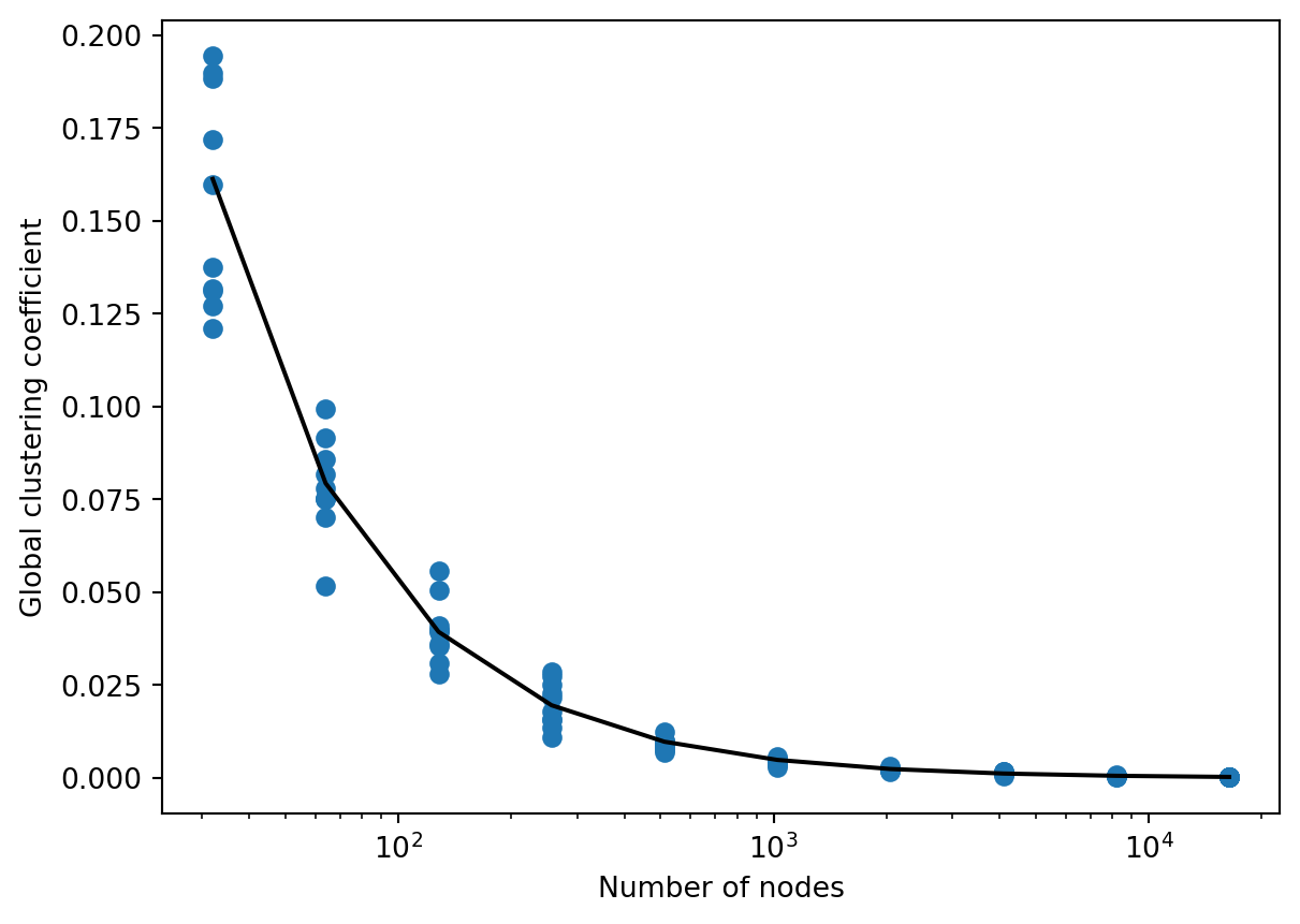
Although the estimate that the global clustering coefficient should be equal to \(p\) was somewhat informal, experimentally it works quite well.
Recall the following definition:
A triangle is an example of a cycle of length \(3\). Our argument about the graph transitivity shows that triangles are rare in sparse \(G(n,p)\) graphs: if I look at any given wedge, the probability that the wedge is completed to form a triangle shrinks to zero with rate \(n^{-1}\). In fact, it is true more generally that cycles of any length are rare in sparse \(G(n,p)\) graphs.
Graphs in which cycles are rare are often called locally tree-like. A tree is a graph without cycles; if cycles are very rare, then we can often use techniques algorithms that are normally guaranteed to only work on trees without running into (too much) trouble.
How far apart are two nodes in \(G(n,p)\)? Again, exactly computing the length of geodesic paths involves some challenging mathematical detail. However, we can get a big-picture view of the situation by asking a slightly different question:
Given two nodes \(i\) and \(j\), what is the expected number of paths of length \(k\) between them?
Let \(R(k)\) denote the number of \(k\)-paths between \(i\) and \(j\). Let \(r(k) = \mathbb{E}[R(k)]\). Let’s estimate \(r(k)\).
First, we know that \(r(1) = p\). For higher values of \(k\), we’ll use the following idea: in order for there to be a path of length \(k\) from \(i\) to \(j\), there must be a node \(\ell\) such that:
There are \(n-2\) possibilities for \(\ell\) (excluding \(i\) and \(j\)), and so we obtain the approximate relation
\[ r(k) \approx (n-2)r(k-1)p\;. \]
Proceeding inductively and approximating \(n-2 \approx n-1\) for \(n\) large, we have the relation
\[ r(k) \approx (n-1)^{k-1}p^{k-1}r(1) = c^{k-1}p \tag{7.1}\]
in the sparse ER model.
Using this result, let’s ask a new question:
What path length \(k\) do I need to allow to be confident that there’s a path of length \(k\) between nodes \(i\) and \(j\)?
Well, suppose we want there to be \(q\) paths. Then, we can solve \(q = c^{k-1}p\) for \(k\), which gives us:
\[ \begin{aligned} q &= c^{k-1}p \\ \log q &= (k-1)\log c + \log p \\ \log q &= (k-1)\log c + \log c - \log n \\ \frac{\log q + \log n}{\log c} &= k \end{aligned} \]
Here, we’ve also approximated \(\log (n-1) \approx \log n\) for \(n\) large. This result tells us that distances between nodes grow very slowly in \(G(n,p)\), roughly at the rate \(\log n\). This is very slow growth. For example, supposing that I want there to be at least one path in expectation (\(q = 1\)), I need to allow \(k = \frac{\log n}{\log c}\). The population of the world is about \(8\times 10^9\), and Newman estimates that an average individual knows around 1,000 other people; that is, \(c = 10^3\) in the world social network. The resulting value of \(k\) here is around 3.3. If on the other hand we wanted to be quite confident that a path exists, we might instead wish to require 1000000 paths, leading to a required path length of roughly 5.3.
In other words, this calculation suggests that, if the world were an ER network, it would be very likely for any two given individuals to be connected by paths of length no longer than 6.
More formal calculations regarding the diameter (length of longest shortest path) of the ER graph confirm that the diameter of the ER graph grows slowly as a function of \(n\).
If you spend some time looking at Equation 7.1, you might find yourself wondering:
Hey, what happens if \(c \leq 1\)?
Indeed, something very interesting happens here. Let’s assume \(c < 1\) (i.e. we’re ignoring the case \(c = 1\)), and estimate the expected number of paths between \(i\) and \(j\) of any length. Using Equation 7.1, we get
\[ \mathbb{E}\left[\sum_{k = 1}^{\infty} R(k)\right] = \sum_{k = 1}^\infty c^{k-1}p = \sum_{k = 0}^\infty c^kp = \frac{p}{1-c}\;. \]
If we now use Markov’s inequality, we find that the probability that there is a path of any length between nodes \(i\) and \(j\) is no larger than \(\frac{p}{1-c}.\) In the sparse regime, we can substitute \(p = \frac{c}{n-1}\) to see that
\[ \frac{c}{(1-c)(n-1)}\rightarrow 0 \text{ as } n \to \infty\;. \]
So, this suggests that, if \(c < 1\), any two nodes are likely to be disconnected! On the other hand, if \(c > 1\), we’ve argued that we can make \(k\) large enough to have high probability of a path of length \(k\) between those nodes.
So, what’s special about \(c = 1\)? This question brings us to one of the first and most beautiful results in the theory of random graphs. To get there, let’s study in a bit more detail the sizes of the connected components of the ER graph.
We’re now going to ask ourselves about the size of a “typical” component in the Erdős–Rényi model. In particular, we’re going to be interested in whether there exists a component that fills up “most” of the graph, or whether components tend to be vanishingly small in relation to the overall graph size.
Our first tool for thinking about this question is the branching process approximation. Informally, a branching process is a process of random generational growth. We’ll get to a formal mathematical definition in a moment, but the easiest way to get insight is to look at a diagram:
We start with a single entity, \(X_0\). Then, \(X_0\) has a random number of “offspring”: \(X_1\) in total. Then, each of those \(X_1\) offspring has some offspring of their own; the total number of these offspring is \(X_2\). The process continues infinitely, although there is always a chance that at some point no more offspring are produced. In this case, we often say that the process “dies out.”
Some of this exposition in this section draws on these notes by David Aldous.
Technically, this is a Galton-Watson branching process, named after the two authors who first proposed it (Watson and Galton 1875).
History note: Galton, one of the founders of modern statistics, was a eugenicist. The cited paper is explicit about its eugenicist motivation: the guiding question was about whether certain family names associated with well-to-do aristocrats were giving way to less elite surnames.
Branching processes create trees – graphs without cycles. The reason that branching processes are helpful when thinking about Erdős–Rényi models is that cycles are rare in Erdős–Rényi random graphs. So, if we can understand the behavior of branching processes, then we can learn something about the Erdős–Rényi random graph as well.
Here’s the particular form of the branching process approximation that we will use:
The idea behind this approximation is:
The mean of a \(\text{Poisson}(c)\) random variable is again \(c\). This implies that \(X_t\), the number of offspring in generation \(t\), satisfies \(\mathbb{E}[X_t] = c^{t}\). It follows that, when \(c < 1\), \(\mathbb{E}[T] = \frac{1}{1-c}\).
Now using Markov’s inequality, we obtain the following results:
So, the probability that the branching process hasn’t yet “died out” decays exponentially with timestep \(t\). In other words, the branching process becomes very likely to die out very quickly. What about the total number of nodes produced in the branching process? Again using Markov’s inequality, we find that
In particular, for \(a\) very large, we are guaranteed that \(\mathbb{P}(T > a)\) is very small.
Summing up, when \(c < 1\), the GW branching process dies out quickly and contains a relatively small number of nodes: \(\frac{1}{1-c}\) in expectation.
If we now translate back to the Erdős–Rényi random graph, the branching process approximation now suggests the following heuristic:
Let’s check this experimentally. The following code block computes the size of the component in an ER graph containing a random node, and averages the result across many realizations. The experimental result is quite close to the theoretical prediction.
import networkx as nx
import numpy as np

def component_size_of_node(n, c):
    G = nx.fast_gnp_random_graph(n, c/(n-1))
    return len(nx.node_connected_component(G, 1))

c = 0.8
sizes = [component_size_of_node(5000, c) for i in range(1000)]

out = f"""
Average over experiments is {np.mean(sizes):.2f}.\n
Theoretical expectation is {1/(1-c):.2f}.
"""

print(out)
Average over experiments is 4.71.

Theoretical expectation is 5.00.
Note that the expected (and realized) component size is very small, even though the graph contains 5,000 nodes!
For this reason, we say that subcritical ER contains only small connected components, in the sense that each component contains approximately 0% of the graph as \(n\) grows large.
This explains our result from earlier about path lengths. The probability that any two nodes have a path between them is the same as the probability that they are on the same connected component. But if every connected component is small, then the probability that two nodes occupy the same one is vanishes.
So far, we’ve argued using the branching process approximation that there is no giant component in the Erdős–Rényi model with \(c < 1\). The theory of branching processes also suggests to us that there could be a giant component when \(c > 1\).
Using our correspondence between components of the ER model and branching processes, this suggests that, if we pick a random node, the component it is in has the potential to be very large. In fact (and this requires some advanced probability to prove formally), when \(c > 1\), there is a giant component. This is our first example of a phase transition.
Examples of phase transitions include freezing, in which a liquid undergoes a qualitative change into a solid in response to a small variation in temperature.
Figure 7.4 shows two sparse ER random graphs on either side of the \(c = 1\) transition. We observe an apparent change in qualitative behavior between the two cases.
import networkx as nx
from matplotlib import pyplot as plt

fig, axarr = plt.subplots(1, 2, figsize = (6, 3))

n = 500
c = [0.7, 1.3]

for i in range(2):
    G = nx.fast_gnp_random_graph(n, c[i]/(n-1))
    nx.draw(G, ax = axarr[i], node_size = 1)
    axarr[i].set(title = f"c = {c[i]}")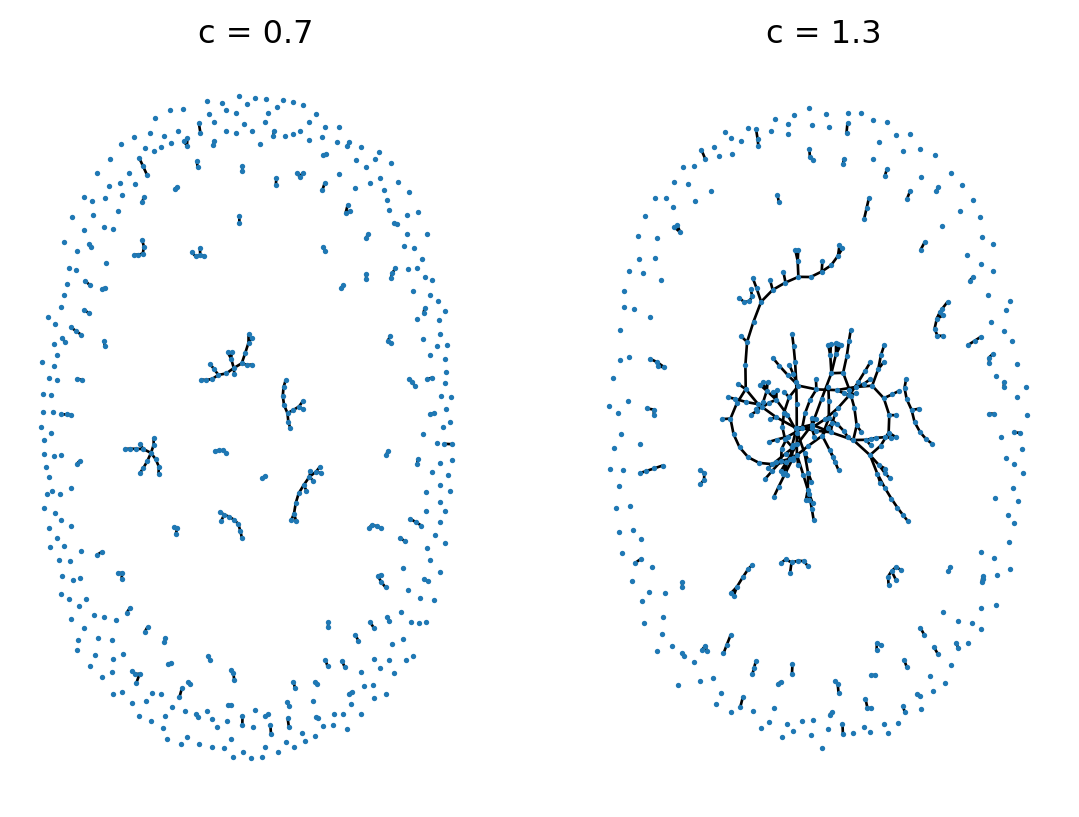
Perhaps surprisingly, while it’s difficult to prove that there is a giant component, it’s not hard at all to estimate its size.
Let \(S\) be the size of the giant component in an Erdős–Rényi random graph, assuming there is one. Then, \(s = S/n\) is the probability that a randomly selected node is in the giant component. Let \(u = 1 - s\) be the probability that a given node is not in the giant component.
Let’s take a random node \(i\), and ask it the probability that it’s in the giant component. Well, one answer to that question is just “\(u\).” On the other hand, we can also answer that question by looking at \(i\)’s neighbors. If \(i\) is not in the giant component, then it can’t be connected to any node that is in the giant component. So, for each other node \(j\neq i\), it must be the case that either:
There are \(n-1\) nodes other than \(i\), and so the probability that \(i\) is not connected to any other node in the giant component is \((1 - p + pu)^{n-1}\). We therefore have the equation
\[ u = (1 - p + pu)^{n-1}\;. \]
Let’s take the righthand side and use \(p = c/(n-1)\): \[ \begin{aligned} u &= (1 - p(1-u))^{n-1} \\ &= \left(1 - \frac{c(1-u)}{n-1}\right)^{n-1}\;. \end{aligned} \] This is a good time to go back to precalculus and remember the limit definition of the function \(e^x\): \[ e^x = \lim_{n \rightarrow \infty}\left(1 + \frac{x}{n}\right)^{n}\;. \] Since we are allowing \(n\) to grow large in our application, we approximate
\[ u \approx e^{-c(1-u)}\;. \] So, now we have a description of the fraction of nodes that aren’t in the giant component. We can get a description of how many nodes are in the giant component by substituting \(s = 1-u\), after which we get the equation we’re really after: \[ s = 1- e^{-cs} \tag{7.2}\]
This equation doesn’t have a closed-form solution for \(s\), but we can still plot it and compare the result to simulations (Figure 7.5). Not bad!
import numpy as np
from matplotlib import pyplot as plt
import networkx as nx

# experiment: compute the size of the largest connected
# component as a function of graph size for a range of mean degrees.

def largest_component(n, p):
    G = nx.fast_gnp_random_graph(n, p)
    S = max(nx.connected_components(G), key=len)
    return len(S) / n

n = 50000
C = np.repeat(np.linspace(0.5, 1.5, 11), 10)
U = np.array([largest_component(n, c/(n-1)) for c in C])

# theory: prediction based on Newman 11.16

S = np.linspace(-.001, .6, 101)
C_theory = -np.log(1-S)/S

# plot the results to compare

plt.plot(C_theory,
         S,
         color = "black",
         label = "Theoretical prediction",
         zorder = -1,
         linestyle = "--")

plt.scatter(C,
            U,
            label = "Experiment",
            facecolor = "steelblue",
            color = "white",
            alpha = 0.8,
            s = 150)

plt.gca().set(xlabel = "Mean degree",
              ylabel = "Proportion of graph in largest component")

plt.legend()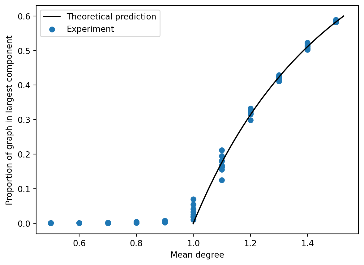
The Erdős–Rényi model \(G(n,p)\) is an important object in random graph theory, and many mathematicians have devoted their careers to studying it. Many of its properties are tractable using tools from probability theory, and it even reproduces some interesting realistic behaviors, such as short path lengths and the existence of a giant component. However, \(G(n,p)\) also has severe limitations as a modeling framework. Since every degree has an approximate Poisson distribution with the same degree, the overall degree distribution is itself Poisson. Many graphs have distinctly non-Poisson degree distributions, and \(G(n,p)\) cannot produce that feature. The scarcity of cycles, especially triangles, in \(G(n,p)\) is also unlike many empirical networks. \(G(n,p)\) also can’t reproduce networks with any kind of modular or community structure.
\(G(n,p)\) is an extremely rich object of mathematical study and an important first model in the study of random graphs. That said, we’ll now move on to models that are more able to reproduce some of the features we observe in empirical networks.
© Heather Zinn Brooks and Phil Chodrow, 2025